39 excel graph data labels different series

How to Rename a Data Series in Microsoft Excel To do this, right-click your graph or chart and click the "Select Data" option. This will open the "Select Data Source" options window. Your multiple data series will be listed under the "Legend Entries (Series)" column. To begin renaming your data series, select one from the list and then click the "Edit" button. Changing data label format for all series in a pivot chart To change data labels format, please perform the following steps: Click the pivot chart > + sign near tthe pivot chart > right click data label of any series > Format Data Series... Besides, to move forward, could you please provide the following information?

Some Data Labels On Series Are Missing - Excel Help Forum For a new thread (1st post), scroll to Manage Attachments, otherwise scroll down to GO ADVANCED, click, and then scroll down to MANAGE ATTACHMENTS and click again. Now follow the instructions at the top of that screen. New Notice for experts and gurus:

Excel graph data labels different series

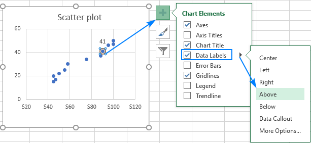
Vary the colors of same-series data markers in a chart In the Format Data Series pane, click the Fill & Line tab, expand Fill, and then do one of the following: To vary the colors of data markers in a single-series chart, select the Vary colors by point check box. To display all data points of a data series in the same color on a pie chart or donut chart, clear the Vary colors by slice check box. excel - Change format of all data labels of a single series at once ... A quick way to solve this is to: Go to the chart and left mouse click on the 'data series' you want to edit. Click anywhere in formula bar above. Don't change anything. Click the 'tick icon' just to the left of the formula bar. Go straight back to the same data series and right mouse click, and choose add data labels. Add Custom Labels to x-y Scatter plot in Excel Step 1: Select the Data, INSERT -> Recommended Charts -> Scatter chart (3 rd chart will be scatter chart) Let the plotted scatter chart be. Step 2: Click the + symbol and add data labels by clicking it as shown below. Step 3: Now we need to add the flavor names to the label. Now right click on the label and click format data labels.

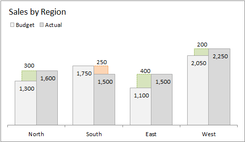
Excel graph data labels different series. Format all data labels at once - MrExcel Message Board My code is below. Select a chart and run it. I have assumed a slope chart with two points per series, any number of series. It removes a legend, if present, adds data labels to each series showing series name and value, ensures data labels are one line only (no word wrap within a label), colors the labels to match the series line, and positions the labels to the left of the left point and to ... Add a DATA LABEL to ONE POINT on a chart in Excel All the data points will be highlighted. Click again on the single point that you want to add a data label to. Right-click and select ' Add data label '. This is the key step! Right-click again on the data point itself (not the label) and select ' Format data label '. You can now configure the label as required — select the content of ... Custom Excel Chart Label Positions - My Online Training Hub Custom Excel Chart Label Positions - Setup. The source data table has an extra column for the 'Label' which calculates the maximum of the Actual and Target: The formatting of the Label series is set to 'No fill' and 'No line' making it invisible in the chart, hence the name 'ghost series': The Label Series uses the 'Value ... Dynamically Label Excel Chart Series Lines - My Online Training Hub This formula ensures that the label for the Actual is at the end of the line, and as the data grows the label moves accordingly. Step 3: Select the first label series. Select the outer edge of the chart to expose the contextual Chart Tools ribbon tabs; Select the Format tab (In Excel 2007 & 2010 it's the Layout tab) Click on the drop down

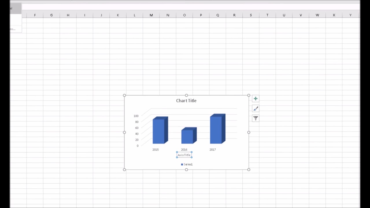
Excel charts: add title, customize chart axis, legend and data labels Click the Chart Elements button, and select the Data Labels option. For example, this is how we can add labels to one of the data series in our Excel chart: For specific chart types, such as pie chart, you can also choose the labels location. For this, click the arrow next to Data Labels, and choose the option you want. Edit titles or data labels in a chart - support.microsoft.com The first click selects the data labels for the whole data series, and the second click selects the individual data label. Right-click the data label, and then click Format Data Label or Format Data Labels. Click Label Options if it's not selected, and then select the Reset Label Text check box. Top of Page Multiple data labels (in separate locations on chart) Re: Multiple data labels (in separate locations on chart) You can do it in a single chart. Create the chart so it has 2 columns of data. At first only the 1 column of data will be displayed. Move that series to the secondary axis. You can now apply different data labels to each series. Attached Files 819208.xlsx‎ (13.8 KB, 264 views) Download How to add data labels from different column in an Excel chart? This method will guide you to manually add a data label from a cell of different column at a time in an Excel chart. 1. Right click the data series in the chart, and select Add Data Labels > Add Data Labels from the context menu to add data labels. 2. Click any data label to select all data labels, and then click the specified data label to select it only in the chart.

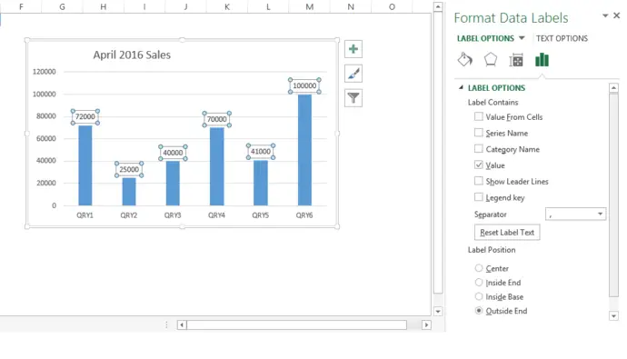
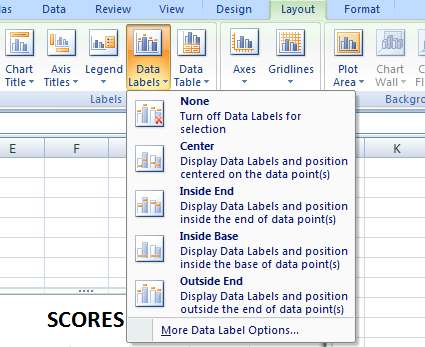
Change the format of data labels in a chart To format data labels, select your chart, and then in the Chart Design tab, click Add Chart Element > Data Labels > More Data Label Options. Click Label Options and under Label Contains, pick the options you want. To make data labels easier to read, you can move them inside the data points or even outside of the chart. How to Create a Graph with Multiple Lines in Excel | Pryor Learning To edit the series labels, follow these steps: Click Select Data button on the Design tab to open the Select Data Source dialog box. Select the series you want to edit, then click Edit to open the Edit Series dialog box. Type the new series label in the Series name: textbox, then click OK. Switch the data rows and columns - Sometimes a different style of chart requires a different layout of the information. Our default line chart makes it difficult to see how each state has performed over ... Multiple Series in One Excel Chart - Peltier Tech Check the settings in the dialo: Values (Y) in rows or columns, series names in first row, categories (X labels) in first column. If Replace Existing Categories is unchecked, the original X labels will remain in the chart. Click OK to update the chart. Add or remove data labels in a chart - support.microsoft.com Click the data series or chart. To label one data point, after clicking the series, click that data point. In the upper right corner, next to the chart, click Add Chart Element > Data Labels. To change the location, click the arrow, and choose an option. If you want to show your data label inside a text bubble shape, click Data Callout.

Advanced Graphs Using Excel : create line plot with error bar plot in excel

Create a multi-level category chart in Excel - ExtendOffice Double click any series in the chart to open the Format Data Series pane. In the pane, change the Gap Width to 0%. 5. Select the spacing1 data series in the chart, go to the Format Data Series pane to configure as follows. 5.1) Click the Fill & Line icon; 5.2) Select No fill in the Fill section. Then these data bars are hidden. 6.

How to Import, Graph, and Label Excel Data in MATLAB: 13 Steps

The Excel Chart SERIES Formula - Peltier Tech Data in an Excel chart is governed by the SERIES formula. This formula is only valid in a chart, not in any worksheet cell, but it can be edited just like any other Excel formula. The SERIES Formula. Select a series in a chart. The source data for that series, if it comes from the same worksheet, is highlighted in the worksheet.

Excel: labels on a scatter chart, read from array - Stack Overflow

How to Change Excel Chart Data Labels to Custom Values? You can change data labels and point them to different cells using this little trick. First add data labels to the chart (Layout Ribbon > Data Labels) Define the new data label values in a bunch of cells, like this: Now, click on any data label. This will select "all" data labels. Now click once again.

Multiple bar charts on one axis in excel - Super User

how to add data labels into Excel graphs - storytelling with data You can download the corresponding Excel file to follow along with these steps: Right-click on a point and choose Add Data Label. You can choose any point to add a label—I'm strategically choosing the endpoint because that's where a label would best align with my design. Excel defaults to labeling the numeric value, as shown below.

Excel - Line Chart

Understanding Excel Chart Data Series, Data Points, and Data Labels Select a data series in a column chart. All columns of the same color are highlighted. Each column is surrounded by a border that includes small dots on the corners. Select the column in the chart to be modified. Only that column is highlighted. Select the Format tab.

highcharts - Optimal display for overlapping series in a line chart - Stack Overflow

Excel 2013: Chart series formatting changes when different series data ... This is without doubt the dumbest "feature" of the new version of Excel. You've probably already figured it out, but, for posterity... Options>Advanced> Chart>Properties follow chart data point for current workbook Uncheck that and you should be golden. cheers, Peter PS I think it's pretty amazing that MS support didn't figure this out.

Excel Formulas Tricks

Individually Formatted Category Axis Labels - Peltier Tech Format the category axis (horizontal axis) so it has no labels. Add data labels to the the dummy series. Use the Below position and Category Names option. Format the dummy series so it has no marker and no line. To format an individual label, you need to single click once to select the set of labels, then single click again to select the ...

Programmatically adding excel data labels in a bar chart - Stack Overflow

How to group (two-level) axis labels in a chart in Excel? Create a Pivot Chart with selecting the source data, and: (1) In Excel 2007 and 2010, clicking the PivotTable > PivotChart in the Tables group on the Insert Tab; (2) In Excel 2013, clicking the Pivot Chart > Pivot Chart in the Charts group on the Insert tab. 2. In the opening dialog box, check the Existing worksheet option, and then select a ...

30 How To Label Points In Excel - Labels For You

XL Chart: Separately align series and value data labels Re: XL Chart: Separately align series and value data labels. You only get one set of data labels per data series. If Excel puts. multiple values within a label, it does so by concatenation, using the. separator you specify. To get multiple labels, you could always add an invisible series (line.

How to add data labels from different column in an Excel chart?

Add a data series to your chart - support.microsoft.com Leaving the dialog box open, click in the worksheet, and then click and drag to select all the data you want to use for the chart, including the new data series. The new data series appears under Legend Entries (Series) in the Select Data Source dialog box. Click OK to close the dialog box and to return to the chart sheet.

November 2018

Add Custom Labels to x-y Scatter plot in Excel Step 1: Select the Data, INSERT -> Recommended Charts -> Scatter chart (3 rd chart will be scatter chart) Let the plotted scatter chart be. Step 2: Click the + symbol and add data labels by clicking it as shown below. Step 3: Now we need to add the flavor names to the label. Now right click on the label and click format data labels.

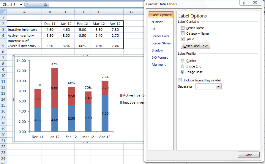
How-to Put Percentage Labels on Top of a Stacked Column Chart - Excel Dashboard Templates

excel - Change format of all data labels of a single series at once ... A quick way to solve this is to: Go to the chart and left mouse click on the 'data series' you want to edit. Click anywhere in formula bar above. Don't change anything. Click the 'tick icon' just to the left of the formula bar. Go straight back to the same data series and right mouse click, and choose add data labels.