40 how to format axis labels in excel
How to format axis labels individually in Excel - SpreadsheetWeb Double-click on the axis you want to format. Double-clicking opens the right panel where you can format your axis. Open the Axis Options section if it isn't active. You can find the number formatting selection under Number section. Select Custom item in the Category list. Type your code into the Format Code box and click Add button. Add axis label in excel | WPS Office Academy 1. First click so you can choose the type of chart where you want to place the axis label. 2. Now click where the chart elements button is located in the right corner of the chart. Then where the expanded menu is located, you must mark the axis titles alternative. 3.
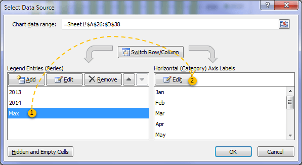
How To Change Y-Axis Values in Excel (2 Methods) | Indeed.com Click "Switch Row/Column". In the dialog box, locate the button in the center labeled "Switch Row/Column". Click on this button to swap the data that appears along the X and Y-axis. Use the preview window in the dialog box to ensure that the data transfers correctly and appears on the correct axis. 4.

How to format axis labels in excel
How do I manually edit the horizontal axis in Excel? The Format Axis window appears. 3. Click on the radio button next to "Specify interval unit," then place your cursor into the small text box next to the button. Type in the interval that you want to use for the X-axis labels. The first axis label displays, then Excel skips labels until the number of your interval, and continues on in this pattern. How to Add Axis Titles in a Microsoft Excel Chart You can either right-click a title and select "Format Axis Title" or double-click one of the titles. At the top of the sidebar, make sure you see Title Options. Then use the three tabs directly below it for Fill & Line, Effects, and Size & Properties to make your adjustments. How to Change the Y Axis in Excel - Alphr Click on the axis that you want to customize. Open the "Format" tab and select "Format Selection." Go to the "Axis Options", click on "Number" and select "Number" from the dropdown selection under...
How to format axis labels in excel. Two-Level Axis Labels (Microsoft Excel) Excel automatically recognizes that you have two rows being used for the X-axis labels, and formats the chart correctly. Since the X-axis labels appear beneath the chart data, the order of the label rows is reversed—exactly as mentioned at the first of this tip. (See Figure 1.) Figure 1. Two-level axis labels are created automatically by Excel. Formatting Long Labels in Excel - PolicyViz Select the axis you want to format and select the Format option in the Paragraph menu. In the ensuing menu, select the Right option in the Alignment drop-down menu. How to Add Axis Label to Chart in Excel - Sheetaki Method 1: By Using the Chart Toolbar. Select the chart that you want to add an axis label. Next, head over to the Chart tab. Click on the Axis Titles. Navigate through Primary Horizontal Axis Title > Title Below Axis. An Edit Title dialog box will appear. In this case, we will input "Month" as the horizontal axis label. Next, click OK. You ... How to Change X-Axis Values in Excel (with Easy Steps) That will bring out the Format Axis option. Then, in the Format Axis option, find Labels. Here the intervals are by default selected Automatically. For our case, we want the interval to be 3. To do so, select Specify interval unit and set it to 3 and press Enter. After pressing Enter, we will have a graph like below.
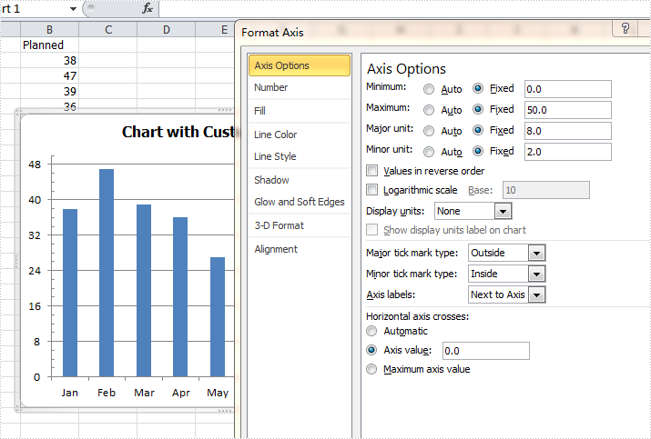
How to Change Axis Scales in Excel Plots (With Examples) To change the scale of the x-axis, simply right click on any of the values on the x-axis. In the dropdown menu that appears, click Format Axis: In the Format Axis panel that appears on the right side of the screen, change the values in the Minimum and Maximum boxes to change the scale of the x-axis. For example, we could change the Maximum ... Modifying Axis Scale Labels (Microsoft Excel) Double-click the axis you want to scale. You should see the Format Axis dialog box. (If double-clicking doesn't work, right-click the axis and choose Format Axis from the resulting Context menu.) Make sure the Number tab is displayed. (See Figure 1.) Figure 1. The Number tab of the Format Axis dialog box. In the Category list, choose Custom. How do I change the X-axis labels in Excel? - Vivu.tv How To Label Axis In Excel? Click the chart, and then click the Chart Design tab. Click Add Chart Element > Axis Titles, and then choose an axis title option. Type the text in the Axis Title box. To format the title, select the text in the title box, and then on the Home tab, under Font, select the formatting that you want. How to Print Labels from Excel - Lifewire Choose Start Mail Merge > Labels . Choose the brand in the Label Vendors box and then choose the product number, which is listed on the label package. You can also select New Label if you want to enter custom label dimensions. Click OK when you are ready to proceed. Connect the Worksheet to the Labels
How to Change the X-Axis in Excel - Alphr Now, right-click on the Horizontal Axis and choose Format Axis… from the menu. Select Axis Options > Labels. Under Interval between labels, select the radio icon next to Specify interval unit and... How to change the position of the secondary Y axis label in Excel Plot ... 1. Right-click the secondary Y-axis label you want to format, and click Format Axis. 2. Under Axis Options, Click the Labels. See the screenshot below There are 4 options: Next to Axis, High, Low, None As for the VBA code you mentioned, unfortunately, due to limited conditions, Microsoft community can only solve concerns about basic use of excel. How to Add Thousand Separator in Excel - Sheetaki First, type an equal sign to start the function. Then, input the TEXT function and select the cell containing the numerical value you want to add a thousand separator. In this case, let's select A2. Finally, input the format "#,###" to add a thousand separator or "#,###.00" if you want to show decimal values. How to make a 3 Axis Graph using Excel? - GeeksforGeeks Double click on the data label of graph2. Step 30: A Format Axis dialogue box appears. Under the Axis Options, set the minimum and maximum with hit and trial. For example, set the minimum to 0 and maximum to 20. Step 31: Similarly Double click, on the secondary axis of graph2. Format Axis dialogue box appears.
34 How To Label Axis In Excel - Labels For You
Excel: How to Create a Bubble Chart with Labels - Statology Step 3: Add Labels. To add labels to the bubble chart, click anywhere on the chart and then click the green plus "+" sign in the top right corner. Then click the arrow next to Data Labels and then click More Options in the dropdown menu: In the panel that appears on the right side of the screen, check the box next to Value From Cells within ...

Excel chart show year intervals on axis - Super User
How to add axis labels in excel | WPS Office Academy Below you will find the steps of how to add axis labels in Excel correctly: 1. The first thing you need to do is select your chart and go to the Chart Design tab. Then click the Add Chart Element dropdown arrow and move your cursor to Axis Titles. Select Primary Horizontal, Primary Vertical, or both from the dropdown menu. 2.

How To Add Axis Labels In Microsoft Excel
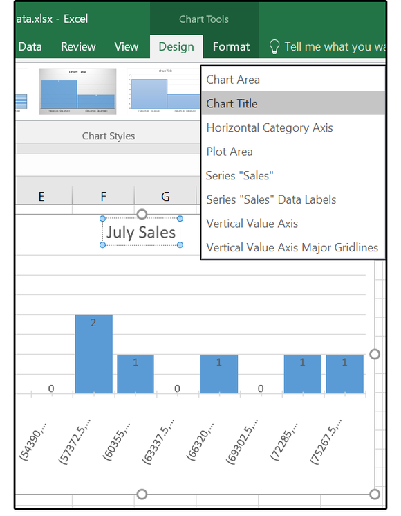
Chart.Axes method (Excel) | Microsoft Docs This example adds an axis label to the category axis on Chart1. VB Copy With Charts ("Chart1").Axes (xlCategory) .HasTitle = True .AxisTitle.Text = "July Sales" End With This example turns off major gridlines for the category axis on Chart1. VB Copy Charts ("Chart1").Axes (xlCategory).HasMajorGridlines = False
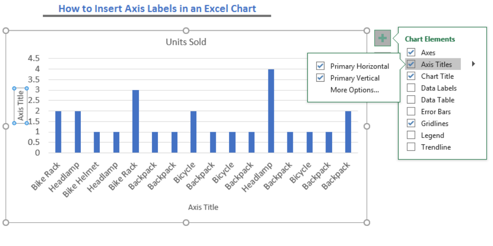
How to Insert Axis Labels In An Excel Chart | Excelchat
How to create a magic quadrant chart in Excel - Data Cornering 1. Select columns with X and Y parameters and insert a scatter chart. 2. Select the horizontal axis of the axis and press shortcut Ctrl + 1. 3. Set the minimum, maximum, and position where the vertical axis crosses. Sometimes it is necessary to leave a gap for the situation when values reach maximum or minimum.
Add Horizontal Category Axis Label Excel
How to Format Data Labels in Excel (with Easy Steps) Then, in the Select Data Source dialog box, click on the Edit option from the Horizontal Axis Labels. In the Axis Labels dialog box, select column B as the Axis label range. Then, click on OK. Finally, click on OK in the Source Data Source dialog box. Finally, we get the following chart. See the screenshot.

How To Add Axis Labels In Microsoft Excel
How do I change the vertical axis values in Excel 2020? The Format Axis window appears. 3. Click on the radio button next to "Specify interval unit," then place your cursor into the small text box next to the button. Type in the interval that you want to use for the X-axis labels. The first axis label displays, then Excel skips labels until the number of your interval, and continues on in this pattern.
Excel Custom Chart Labels • My Online Training Hub
How to Create and Customize a Waterfall Chart in Microsoft Excel To fix this, double-click the chart to display the Format sidebar. Select the bar for the total by clicking it twice. Click the Series Options tab in the sidebar and expand Series Options if necessary. Check the box for "Set as Total." Then, do the same for the other total.
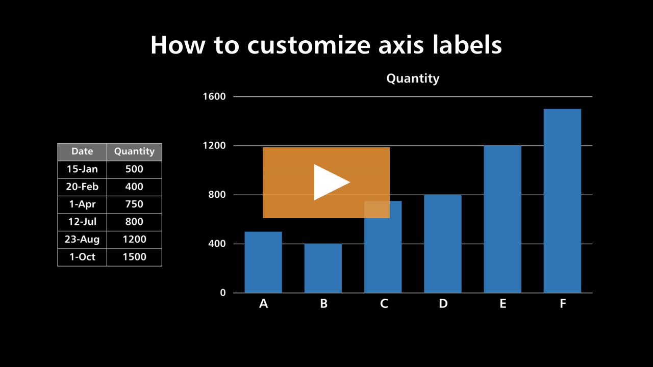
How to format the chart axis labels in Excel 2010 - YouTube
Axis.TickLabels property (Excel) | Microsoft Docs Returns a TickLabels object that represents the tick-mark labels for the specified axis. Read-only. Syntax. expression.TickLabels. expression A variable that represents an Axis object. Example. This example sets the color of the tick-mark label font for the value axis on Chart1. Charts("Chart1").Axes(xlValue).TickLabels.Font.ColorIndex = 3 ...
How to format axis for Excel chart in C#
Excel Waterfall Chart: How to Create One That Doesn't Suck Click inside the data table, go to " Insert " tab and click " Insert Waterfall Chart " and then click on the chart. Voila: OK, technically this is a waterfall chart, but it's not exactly what we hoped for. In the legend we see Excel 2016 has 3 types of columns in a waterfall chart: Increase. Decrease.
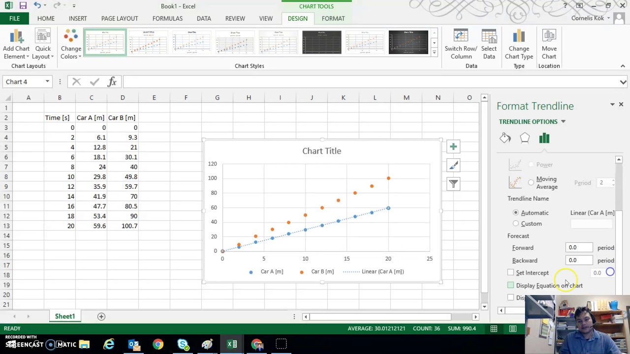
Microsoft Excel - Creating a Scatter Plot with trend line and axis labels - YouTube
Format Chart Axis in Excel - Axis Options Analyzing Format Axis Pane Right-click on the Vertical Axis of this chart and select the "Format Axis" option from the shortcut menu. This will open up the format axis pane at the right of your excel interface. Thereafter, Axis options and Text options are the two sub panes of the format axis pane.

Excel Charts | Real Statistics Using Excel
How to Change the Y Axis in Excel - Alphr Click on the axis that you want to customize. Open the "Format" tab and select "Format Selection." Go to the "Axis Options", click on "Number" and select "Number" from the dropdown selection under...
35 How To Label Chart Axis In Excel - Label Design Ideas
How to Add Axis Titles in a Microsoft Excel Chart You can either right-click a title and select "Format Axis Title" or double-click one of the titles. At the top of the sidebar, make sure you see Title Options. Then use the three tabs directly below it for Fill & Line, Effects, and Size & Properties to make your adjustments.

How To Label Axis On Excel 2016 - Pensandpieces
How do I manually edit the horizontal axis in Excel? The Format Axis window appears. 3. Click on the radio button next to "Specify interval unit," then place your cursor into the small text box next to the button. Type in the interval that you want to use for the X-axis labels. The first axis label displays, then Excel skips labels until the number of your interval, and continues on in this pattern.
How to Move X Axis Labels from Top to Bottom - ExcelNotes
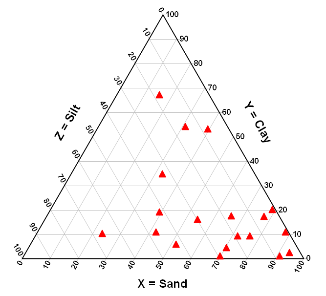
DPlot Triangle Plot
Excel 2016 charts: How to use the new Pareto, Histogram, and Waterfall formats | PCWorld
Post a Comment for "40 how to format axis labels in excel"