40 how to add two data labels in excel pie chart

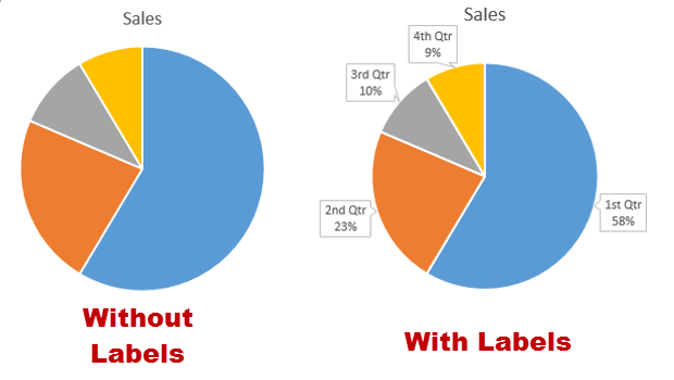
How to Combine or Group Pie Charts in Microsoft Excel Click on the first chart and then hold the Ctrl key as you click on each of the other charts to select them all. Click Format > Group > Group. All pie charts are now combined as one figure. They will move and resize as one image. Choose Different Charts to View your Data Pie of Pie Chart in Excel - Inserting, Customizing, Formatting To add the data labels:- Select the chart and click on + icon at the top right corner of chart. Mark the check box containing data labels. Formatting Data Labels Consequently, this is going to insert default data labels on the chart.

How to make a pie chart in Excel » App Authority 2. We've selected the 2-D Pie option for this example. You should see your graph appear on the spreadsheet with an automatic title and legend. 3. If you want to add labels to your pie chart, you first have to right-click on the chart to open the menu. From the menu, select the Add Data Labels option to display your data within the pie ...

How to add two data labels in excel pie chart

How to Add Data Labels to an Excel 2010 Chart - dummies Use the following steps to add data labels to series in a chart: Click anywhere on the chart that you want to modify. On the Chart Tools Layout tab, click the Data Labels button in the Labels group. None: The default choice; it means you don't want to display data labels. Center to position the data labels in the middle of each data point. How to add data labels from different column in an Excel chart? Right click the data series in the chart, and select Add Data Labels > Add Data Labels from the context menu to add data labels. 2. Click any data label to select all data labels, and then click the specified data label to select it only in the chart. 3. Pie Chart Examples | Types of Pie Charts in Excel ... - EDUCBA Now our task is to add the Data series to the PIE chart divisions. Click on the PIE chart so that the chart will get a highlight, as shown below. Right-click and choose the “Add Data Labels “option for additional drop-down options.

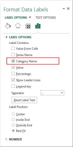
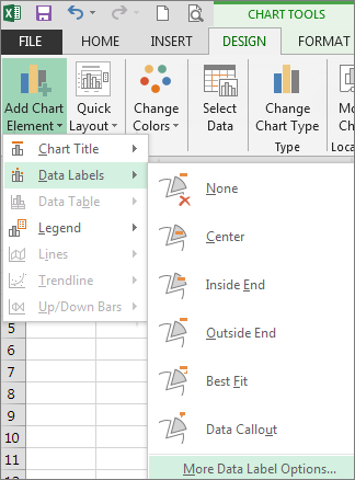
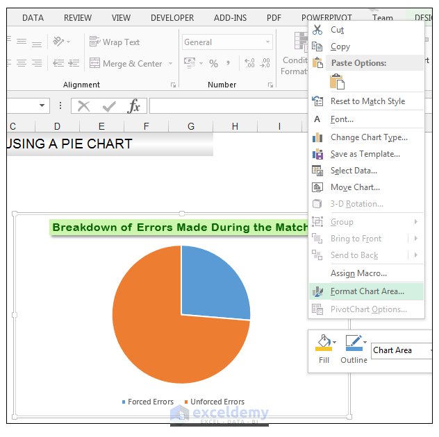
How to add two data labels in excel pie chart. Creating Pie Chart and Adding/Formatting Data Labels (Excel) Creating Pie Chart and Adding/Formatting Data Labels (Excel) Creating Pie Chart and Adding/Formatting Data Labels (Excel) Pivot Chart Data Label Help Needed - Microsoft Community Open the Excel file with Pivot Chart and enabled with Data Labels> Click on the Labels displayed in the Chart> Right-click> Click Format Data Labels> Label Options> Number> In the Category, select the format as per your requirement. Here is the reference article: Change the format of data labels in a chart. Add or remove data labels in a chart - support.microsoft.com Click the data series or chart. To label one data point, after clicking the series, click that data point. In the upper right corner, next to the chart, click Add Chart Element > Data Labels. To change the location, click the arrow, and choose an option. If you want to show your data label inside a text bubble shape, click Data Callout. Edit titles or data labels in a chart - support.microsoft.com On a chart, click one time or two times on the data label that you want to link to a corresponding worksheet cell. The first click selects the data labels for the whole data series, and the second click selects the individual data label. Right-click the data label, and then click Format Data Label or Format Data Labels.

How to Create and Format a Pie Chart in Excel - Lifewire To add data labels to a pie chart: Select the plot area of the pie chart. Right-click the chart. Select Add Data Labels . Select Add Data Labels. In this example, the sales for each cookie is added to the slices of the pie chart. Change Colors Possible to add second data label to pie chart? - Excel Help Forum Re: Possible to add second data label to pie chart? Create the composite label in a worksheet column by concatenating the data in other cells and the nextline character, CHR (10). Now, use this composite label column as the source for Rob Bovey's add-in. -- Regards, Tushar Mehta Excel, PowerPoint, and VBA add-ins, tutorials adding decimal places to percentages in pie charts Hello DV_1956. I am V. Arya, Independent Advisor, to work with you on this issue. Right click on your % label - Format Data labels. Beneath Number choose percentage as category. Report abuse. 42 people found this reply helpful. ·. Was this reply helpful? Add a DATA LABEL to ONE POINT on a chart in Excel All the data points will be highlighted. Click again on the single point that you want to add a data label to. Right-click and select ' Add data label '. This is the key step! Right-click again on the data point itself (not the label) and select ' Format data label '. You can now configure the label as required — select the content of ...

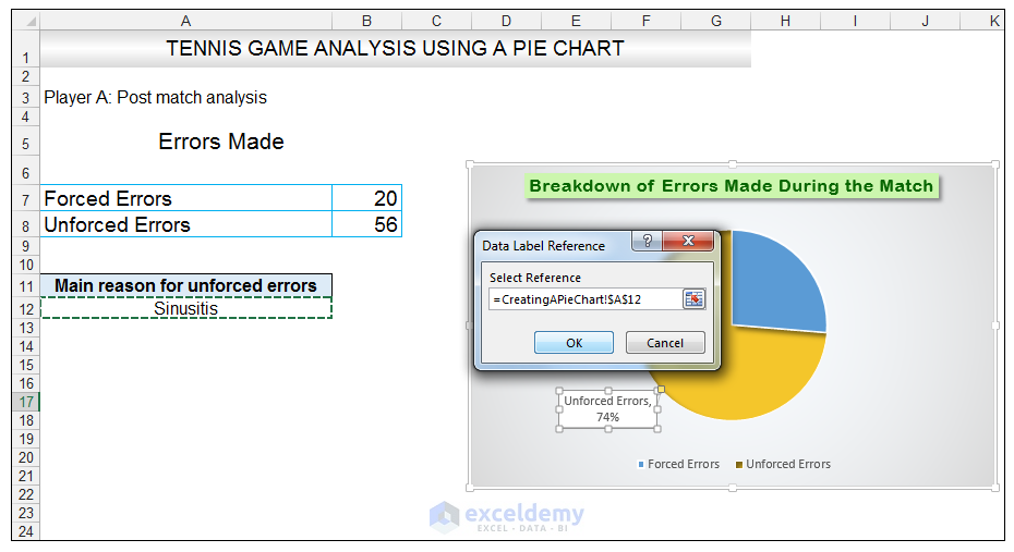
How to Make a Pie Chart in Excel & Add Rich Data Labels to The Chart! 8) With the one data point still selected, right-click this data point, and select Add Data Label>Add Data Callout as shown below. 9) Select only this data label and right-click and choose Insert Data Label Field as shown below. 10) Select [Cell] Choose Cell from the options. How to Create Bar of Pie Chart in Excel? Step-by-Step To be able to see the actual percentage of each portion/ category, adding data labels would be quite helpful. To add and format data labels to portions in your Bar of pie chart, follow the steps below: Click anywhere on the blank area of the chart. You will see three icons appear to the right side of the chart, as shown below: How to add Axis Labels (X & Y) in Excel & Google Sheets How to Add Axis Labels (X&Y) in Excel. Graphs and charts in Excel are a great way to visualize a dataset in a way that is easy to understand. The user should be able to understand every aspect about what the visualization is trying to show right away. As a result, including labels to the X and Y axis is essential so that the user can see what ... How to Create Multi-Category Charts in Excel? - GeeksforGeeks Step 1: Insert the data into the cells in Excel. Now select all the data by dragging and then go to "Insert" and select "Insert Column or Bar Chart". A pop-down menu having 2-D and 3-D bars will occur and select "vertical bar" from it. Select the cell -> Insert -> Chart Groups -> 2-D Column.

How can someone create a pie chart with 2 variables in MS Excel? - Quora

Create two data labels in pie chart? - MrExcel Message Board You have already figured out how to add an image that fills the sector of the pie chart but as far as I know you cannot add an icon or image over the actual pie chart sector, in such a way that it adjusts with the values. If you add it as a static image next to the legend, at least the legend does not move when the values change. Paul.

Excel 3-D Pie charts - Microsoft Excel 2013

Office: Display Data Labels in a Pie Chart - Tech-Recipes 3. In the Chart window, choose the Pie chart option from the list on the left. Next, choose the type of pie chart you want on the right side. 4. Once the chart is inserted into the document, you will notice that there are no data labels. To fix this problem, select the chart, click the plus button near the chart's bounding box on the right ...

Office: Display Data Labels in a Pie Chart

How to add or move data labels in Excel chart? - ExtendOffice To add or move data labels in a chart, you can do as below steps: In Excel 2013 or 2016. 1. Click the chart to show the Chart Elements button .. 2. Then click the Chart Elements, and check Data Labels, then you can click the arrow to choose an option about the data labels in the sub menu.See screenshot:

How to Make a Pie Chart in Excel & Add Rich Data Labels to The Chart!

Adding data labels to a pie chart - Excel General - OzGrid Re: Adding data labels to a pie chart. Thanks again, norie. Really appreciate the help. I tried recording a macro while doing it manually (before my first post). But it didn't record anything about labels, much less making them bold.

How to Make a Pie Chart in Excel & Add Rich Data Labels to The Chart!

How do I add leader lines for a pie chart? : excel Press J to jump to the feed. Press question mark to learn the rest of the keyboard shortcuts

How to Create a Pie Chart in Excel | onsite-training.com

How do I label a pie chart? - Blfilm.com Select Add Data Labels. Select Add Data Labels. In this example, the sales for each cookie is added to the slices of the pie chart. How do you show Percentages on a pie chart in Matlab? Labels with Percentages and Text x = [1,2,3]; p = pie(x); Get the percent contributions for each pie slice from the String properties of the text objects.

Microsoft Excel Tutorials: Add Data Labels to a Pie Chart

Add data labels and callouts to charts in Excel 365 - EasyTweaks.com Step #1: After generating the chart in Excel, right-click anywhere within the chart and select Add labels . Note that you can also select the very handy option of Adding data Callouts.

SQL & BI Learning: Pie Chart with data labels outside in ssrs

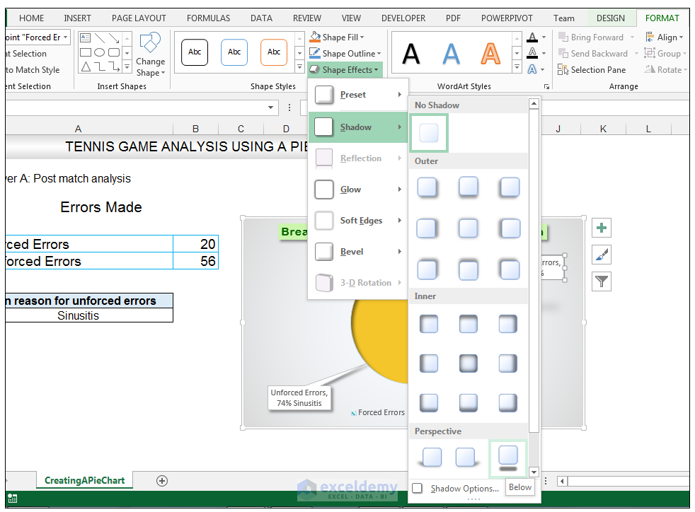
How to add two data labels for the same data on a pie chart? Consider using two sheets, a "Calculation" sheet and your "Dashboard" sheet. Create your pie graph as usual on the "Dashboard" sheet, but remove all labels. Adjust the colors as desired. On your "Calculation sheet, create the text for your percentage label and your ratio label. For example, the first pie chart charts the data 46 and 76.

Understanding Excel Chart Data Series, Data Points, and Data Labels

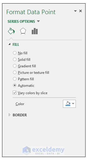
How to Edit Pie Chart in Excel (All Possible Modifications) This will add two tabs named Chart Design and Format in the ribbon. Secondly, go to the Chart Design tab from the ribbon. Subsequently, click on the Change Colors tool. At this time, choose any color you want for your pie chart. Therefore, you will see that you have made edits in your pie chart color successfully according to your choice.

Formatting data labels and printing pie charts on Excel for Mac 2019 - - Microsoft Community

Create a pie chart from distinct values in one column by ... On the PivotTable Field List drag Country to Row Labels and Count to Values if Excel doesn't automatically. Now select the pivot table data and create your pie chart as usual. P.S. I use the pivot table for I update the data on a regular basis, then I just replace the "Country" data and refresh the pivot table.

Insert a pie chart in Excel - Excel

Pie Chart in Excel | How to Create Pie Chart - EDUCBA Step 1: Select the data to go to Insert, click on PIE, and select 3-D pie chart. Step 2: Now, it instantly creates the 3-D pie chart for you. Step 3: Right-click on the pie and select Add Data Labels. This will add all the values we are showing on the slices of the pie.

Lesson 38 - How to add DATA LABELS to charts in Excel | Change colour of pie-chart segments in ...

How to Add Gridlines in a Chart in Excel? 2 Easy Ways! Let us now see two ways to insert major and minor gridlines in Excel. Method 1: Using the Chart Elements Button to Add and Format Gridlines. The Chart Elements button appears to the right of your chart when it is selected. This button allows you to add, change or remove chart elements like the title, legend, gridlines, and labels.

Excel 2010 Secondary Axis Bar Chart Overlap - secondary vertical axis user friendlyhow to show ...

Format data series excel pie chart How to draw pie charts in Excel. In this article, TipsMake will use Excel 2016 to demonstrate how to draw pie chart in Excel.Suppose you have a data table as shown below, need to insert pie chart.Step 1: You perform the highlighting of the data you need to draw a pie chart.Step 2: Then go to the Insert tab-> select the icon of the pie chart.... Answer: A pie chart isn't meant to show two ...

How to Create Excel Pie Charts & Add Rich Data Labels to The Chart!

Understanding Excel Chart Data Series, Data Points, and Data ... Sep 19, 2020 · Add Emphasis With a Combo Chart . Another option for emphasizing different types of information in a chart is to display two or more chart types in a single chart, such as a column chart and a line graph. You could use this approach when the graphed values vary widely or when graphing different types of data.

tableau quick filters – Books guides

How do you make a pie chart in Excel with two sets of data? Can you add two data labels in Excel pie chart? This method will introduce a solution to add all data labels from a different column in an Excel chart at the same time. Please do as follows: 1. Right click the data series in the chart, and select Add Data Labels > Add Data Labels from the context menu to add data labels.

How to Make a Pie Chart in Excel & Add Rich Data Labels to The Chart!

Format data series excel pie chart - znkszm.la-coquilla.nl The pie chart in Excel can convert a row or column of data. Microsoft suggests a pie chart works best when: You only have one data series.. Figure 4. Pie of pie chart. We can launch Format Data Series by right-clicking the chart and selecting from the menu. Figure 5. Format Data Series option. We can then customize in Series Options. Example.

Share :