43 chart data labels excel
Sunburst Chart is not displaying 'data labels' completely Answer. Thank you for the reply. To meet your requirement, you could try the following two ways: In the Area chart, you could manually move the data labels to the position you want. Or you could try to use Combo chart in the Excel, below is the result (I will send you the sample file in the Private Message ): * Beware of scammers posting fake ... Use a screen reader to add a title, data labels, and a legend to a ... Select the chart that you want to work with. To open the Add Chart Element menu, press Alt+J, C, A. To add data callout labels to the chart, press D and then U. Tip: To remove data labels, select the chart, and then press Alt+J, C, A, D, and then N. Add a legend to a chart Legends help you to quickly understand data relationships in a chart.
How to Customize Your Excel Pivot Chart Data Labels - dummies If you want to label data markers with a category name, select the Category Name check box. To label the data markers with the underlying value, select the Value check box. In Excel 2007 and Excel 2010, the Data Labels command appears on the Layout tab. Also, the More Data Labels Options command displays a dialog box rather than a pane.

Chart data labels excel
Excel tutorial: How to use data labels Data labels are used to display source data in a chart directly. They normally come from the source data, but they can include other values as well, as we'll see in in a moment. Generally, the easiest way to show data labels to use the chart elements menu. When you check the box, you'll see data labels appear in the chart. How to Use Cell Values for Excel Chart Labels Select the chart, choose the "Chart Elements" option, click the "Data Labels" arrow, and then "More Options." Uncheck the "Value" box and check the "Value From Cells" box. Select cells C2:C6 to use for the data label range and then click the "OK" button. The values from these cells are now used for the chart data labels. Add or remove data labels in a chart - support.microsoft.com Click the data series or chart. To label one data point, after clicking the series, click that data point. In the upper right corner, next to the chart, click Add Chart Element > Data Labels. To change the location, click the arrow, and choose an option. If you want to show your data label inside a text bubble shape, click Data Callout.
Chart data labels excel. Edit titles or data labels in a chart - support.microsoft.com Right-click the data label, and then click Format Data Label or Format Data Labels. Click Label Options if it's not selected, and then select the Reset Label Text check box. Top of Page Reestablish a link to data on the worksheet On a chart, click the label that you want to link to a corresponding worksheet cell. Excel charts: add title, customize chart axis, legend and data labels ... Click the Chart Elements button, and select the Data Labels option. For example, this is how we can add labels to one of the data series in our Excel chart: For specific chart types, such as pie chart, you can also choose the labels location. For this, click the arrow next to Data Labels, and choose the option you want. How to create Custom Data Labels in Excel Charts Create the chart as usual. Add default data labels. Click on each unwanted label (using slow double click) and delete it. Select each item where you want the custom label one at a time. Press F2 to move focus to the Formula editing box. Type the equal to sign. Now click on the cell which contains the appropriate label. Excel.ChartDataLabel class - Office Add-ins | Microsoft Docs This connects the add-in's process to the Office host application's process. Represents the format of chart data label. String value that represents the formula of chart data label using A1-style notation. Returns the height, in points, of the chart data label. Value is null if the chart data label is not visible.
Excel: How to Create a Bubble Chart with Labels - Statology To add labels to the bubble chart, click anywhere on the chart and then click the green plus "+" sign in the top right corner. Then click the arrow next to Data Labels and then click More Options in the dropdown menu: In the panel that appears on the right side of the screen, check the box next to Value From Cells within the Label Options group: How To Use Dynamic Data Labels To Create Interactive Excel Charts Insert An Interactive Line Chart With Dynamic Data Labels Select the data and insert a combo chart. For combo, chart go to the Insert → Charts → Combo Charts Now make a selection for the Line Chart for revenue data and a Line Chart With Markers For Data Labels. Now select the Data Label Line and remove fill color from it. Add a DATA LABEL to ONE POINT on a chart in Excel Steps shown in the video above: Click on the chart line to add the data point to. All the data points will be highlighted. Click again on the single point that you want to add a data label to. Right-click and select ' Add data label ' This is the key step! Right-click again on the data point itself (not the label) and select ' Format data label '. Excel.ChartDataLabels class - Office Add-ins | Microsoft Docs excel Represents a collection of all the data labels on a chart point. Extends OfficeExtension.ClientObject Remarks [ API set: ExcelApi 1.1 ] Properties Methods Property Details auto Text Specifies if data labels automatically generate appropriate text based on context. autoText: boolean; Property Value boolean Remarks [ API set: ExcelApi 1.8 ]
Excel Charts - Aesthetic Data Labels - Tutorials Point Data labels stay in place, even when you switch to a different type of chart. You can also connect the data labels to their data points with leader lines on all charts. Here, we will use a Bubble chart to see the formatting of data labels. Data Label Positions. To place the data labels in the chart, follow the steps given below. How to add total labels to stacked column chart in Excel? Select the source data, and click Insert > Insert Column or Bar Chart > Stacked Column. 2. Select the stacked column chart, and click Kutools > Charts > Chart Tools > Add Sum Labels to Chart. Then all total labels are added to every data point in the stacked column chart immediately. Create a stacked column chart with total labels in Excel Create Dynamic Chart Data Labels with Slicers - Excel Campus Typically a chart will display data labels based on the underlying source data for the chart. In Excel 2013 a new feature called "Value from Cells" was introduced. This feature allows us to specify the a range that we want to use for the labels. Since our data labels will change between a currency ($) and percentage (%) formats, we need a ... How to add data labels from different column in an Excel chart? Right click the data series in the chart, and select Add Data Labels > Add Data Labels from the context menu to add data labels. 2. Click any data label to select all data labels, and then click the specified data label to select it only in the chart. 3.

How to Change Excel Chart Data Labels to Custom Values?
Move data labels - support.microsoft.com Right-click the selection > Chart Elements > Data Labels arrow, and select the placement option you want. Different options are available for different chart types. For example, you can place data labels outside of the data points in a pie chart but not in a column chart.

How to Create a Geographical Map Chart in Microsoft Excel
Add / Move Data Labels in Charts - Excel & Google Sheets We'll start with the same dataset that we went over in Excel to review how to add and move data labels to charts. Add and Move Data Labels in Google Sheets Double Click Chart Select Customize under Chart Editor Select Series 4. Check Data Labels 5. Select which Position to move the data labels in comparison to the bars.
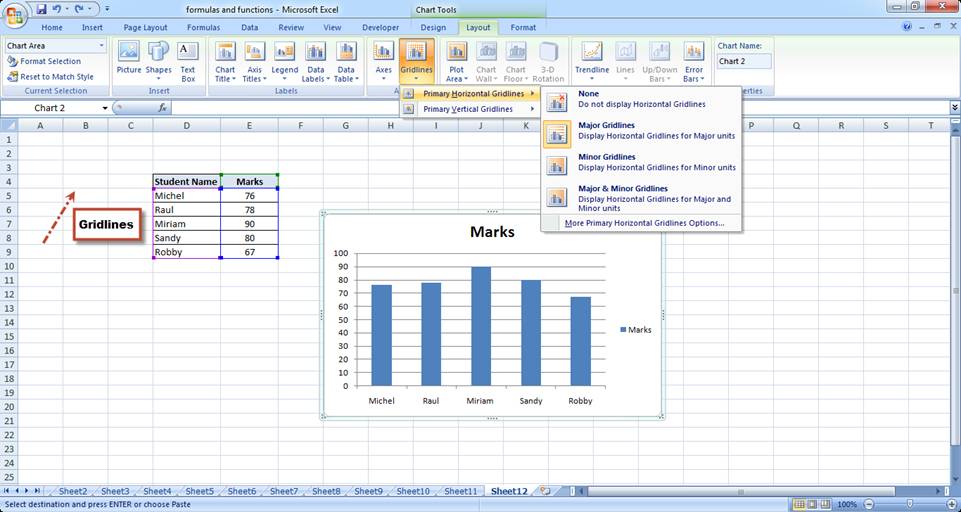
Basic Excel Chart Formatting - MS Excel Charting Tutorial Part 4 | Vertical Horizons
How do I add additional labels to an excel chart? - Stack Overflow I've got a chart in excel and I'd like to add additional labels to it. In the below example I want to add "Inadequate" next to the 34s, "Inconsistent" next to the 42 and so on. Ideally, I'd like to be able to tweek how the floating text looks. I've tried adding an extra row in my data below, but it just messes up the whole chart or isn't useful.
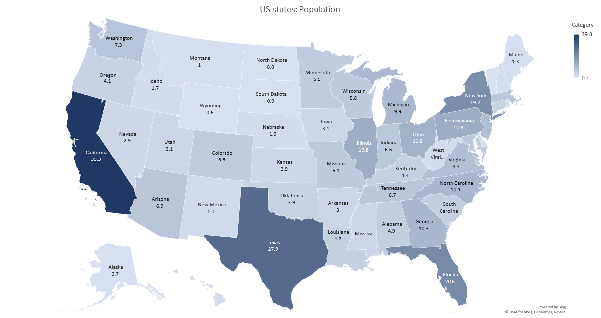
Excel map chart
Custom Chart Data Labels In Excel With Formulas Select the chart label you want to change. In the formula-bar hit = (equals), select the cell reference containing your chart label's data. In this case, the first label is in cell E2. Finally, repeat for all your chart laebls. If you are looking for a way to add custom data labels on your Excel chart, then this blog post is perfect for you.
![Custom Data Labels with Colors and Symbols in Excel Charts – [How To] - KING OF EXCEL](https://pakaccountants.com/wp-content/uploads/2014/09/data-label-chart-7.gif)
Custom Data Labels with Colors and Symbols in Excel Charts – [How To] - KING OF EXCEL
Chart.ApplyDataLabels method (Excel) | Microsoft Docs For the Chart and Series objects, True if the series has leader lines. Pass a Boolean value to enable or disable the series name for the data label. Pass a Boolean value to enable or disable the category name for the data label. Pass a Boolean value to enable or disable the value for the data label.
How-to Use Data Labels from a Range in an Excel Chart - Excel Dashboard Templates
How to add or move data labels in Excel chart? - ExtendOffice In Excel 2013 or 2016 1. Click the chart to show the Chart Elements button . 2. Then click the Chart Elements, and check Data Labels, then you can click the arrow to choose an option about the data labels in the sub menu. See screenshot: In Excel 2010 or 2007 1. click on the chart to show the Layout tab in the Chart Tools group. See screenshot: 2.

Creating Pie Chart and Adding/Formatting Data Labels (Excel) - YouTube
How to Change Excel Chart Data Labels to Custom Values? Go to Formula bar, press = and point to the cell where the data label for that chart data point is defined. Repeat the process for all other data labels, one after another. See the screencast. Points to note: This approach works for one data label at a time. So if you have a large chart, you are in for a lot of clicks and manic mouse maneuvering.

How-to Use Data Labels from a Range in an Excel Chart - Excel Dashboard Templates
Change the format of data labels in a chart To get there, after adding your data labels, select the data label to format, and then click Chart Elements > Data Labels > More Options. To go to the appropriate area, click one of the four icons ( Fill & Line, Effects, Size & Properties ( Layout & Properties in Outlook or Word), or Label Options) shown here.

Do My Excel Blog: How to design a multiple clustered bar chart series in Excel
How to Add Labels to Scatterplot Points in Excel - Statology Step 1: Create the Data First, let's create the following dataset that shows (X, Y) coordinates for eight different groups: Step 2: Create the Scatterplot Next, highlight the cells in the range B2:C9. Then, click the Insert tab along the top ribbon and click the Insert Scatter (X,Y) option in the Charts group. The following scatterplot will appear:
![Custom Data Labels with Colors and Symbols in Excel Charts - [How To] - PakAccountants.com](https://pakaccountants.com/wp-content/uploads/2014/09/data-label-chart-4.gif)
Custom Data Labels with Colors and Symbols in Excel Charts - [How To] - PakAccountants.com
Adding rich data labels to charts in Excel 2013 - Microsoft 365 Blog Putting a data label into a shape can add another type of visual emphasis. To add a data label in a shape, select the data point of interest, then right-click it to pull up the context menu. Click Add Data Label, then click Add Data Callout . The result is that your data label will appear in a graphical callout.

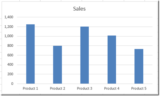
How to Make Charts and Graphs in Excel | Smartsheet
Add or remove data labels in a chart - support.microsoft.com Click the data series or chart. To label one data point, after clicking the series, click that data point. In the upper right corner, next to the chart, click Add Chart Element > Data Labels. To change the location, click the arrow, and choose an option. If you want to show your data label inside a text bubble shape, click Data Callout.
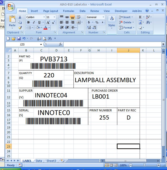
Label Template Excel | printable label templates
How to Use Cell Values for Excel Chart Labels Select the chart, choose the "Chart Elements" option, click the "Data Labels" arrow, and then "More Options." Uncheck the "Value" box and check the "Value From Cells" box. Select cells C2:C6 to use for the data label range and then click the "OK" button. The values from these cells are now used for the chart data labels.
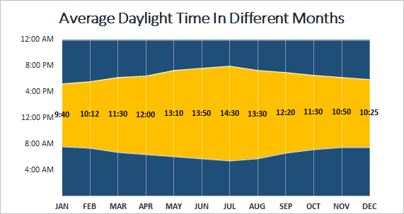
Create Sunrise Chart in Excel
Excel tutorial: How to use data labels Data labels are used to display source data in a chart directly. They normally come from the source data, but they can include other values as well, as we'll see in in a moment. Generally, the easiest way to show data labels to use the chart elements menu. When you check the box, you'll see data labels appear in the chart.

Show Trend Arrows in Excel Chart Data Labels
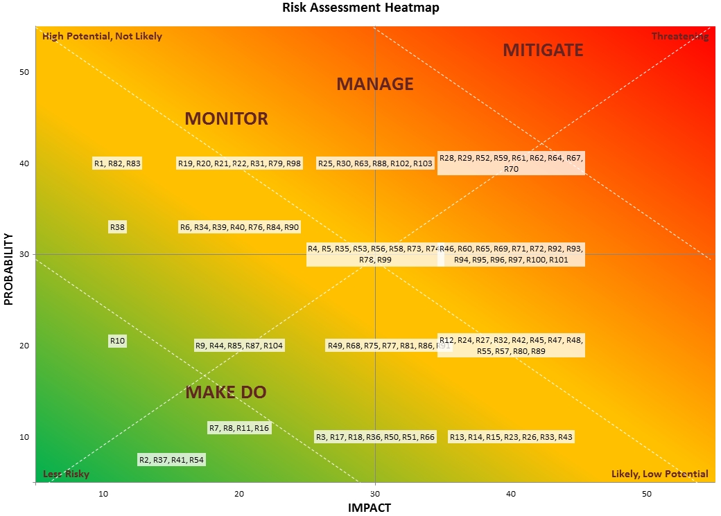
How to Create a Risk Heatmap in Excel - Part 2 - Risk Management Guru
Post a Comment for "43 chart data labels excel"